1. Reading in the Data
A list of all dicom files in the requested folder was determined by searching for all files in the directory ending in ”.dcm.” The file names and slice location from the header files for each file was stored in a 2 dimensional matrix. The matrix was sorted by the slice location to determine the order of the files in the CT image. This successfully read in the files in the appropriate order as was shown later by visualizing the image stack with imtool3D. This portion of the algorithm was slow and could be improved by developing a faster sorting algorithm.
2. Creating Volume of CT
Initially, a 3 dimensional matrix was creating with sizing determined by the pixel height/width infor- mation from the first image in the file and the number of dicom files in the folder. Since the size was determined dynamically, this algorithm is applicable to any number and any size of images. Using the predetermined file order, the image information for each slice was stored in the matrix. The images were successfully read as shown by Figure 6(a).
The pixel intensities were then normalized using standard Z-score normalization. After normalization, the pixel intensities were separated into light and dark groups of pixels (see Figure 2). There were many other alternatives to normalizing the pixel intensities, but this method enabled successful segmentation as shown by the final image of the segmented lung.
3. Thresholding and Segmentation
A black and white representation of the CT images was generated by using Otsu’s method was used to segment the image into foreground and background pixels (see middle panel of Figure 3). In order to select only the middle lung, all pixels connected to the four corners of the image were filtered out of the final segmented image (see right panel of Figure 3).
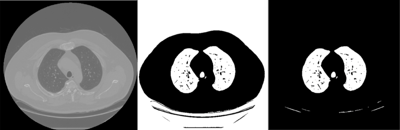 Figure 3: Segmented CT Slice
Otsu’s method is a very quick way of thresholding and worked fairly well for this segmentation since the pixel intensities were approximately bimodal (Figure 2). The method successfully segmented the lung from the majority of the objects in the image, but the segmented image still contained non-lung objects and was missing many of the blood vessels in the center of the lung. Alternative methods that incorporate spatial information and use local thresholding may improve this initial segmentation.
4. Volume Filtering
Next the extraneous objects that are not part of the lung (see lines beneath the lung in the middle and right panels of Figure 3) were removed. This was done by determining the size of all connected objects in the image and filtering all except for the largest object in the image. This was successful because the lung happens to be the largest continuous object in the image, but this method may not work for other tissues in the body. In addition, the trachea remained in the image because it is roughly the same intensity as the lung and is connected to the lung. A slice of the volume filtered lung CT with remaining trachea can be see in Figure 4.
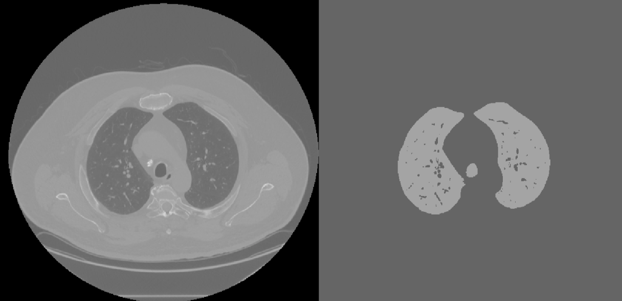 Figure 4: Volume Filtered CT Slice
5. Trachea Removal and Image Smoothing
Morphological closing was used to re-incorporate blood vessels into the segmented image by filling in edges below a certain size. The trachea was then removed by eliminating objects below a certain size in the image. The size of the elements used for trachea removal and image smoothing were were disks of size 5 and 12, respectively. This smoothing incorporated the
While these methods worked successfully for this set of CT images (Figure 5), they required manual tuning and cannot be performed automatically for any set of CT images. This is an area where the algorithm could be improved by developing automatic methods. Its possible that the size of the disks used could be selected by calculating dimensions of the trachea and edges in the image.
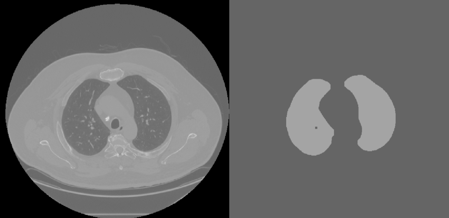 Figure 5: Smoothed CT with Trachea Removed
6. Scatterplot Rendering
In order to perform a basic 3D rendering of the segmented image, isosurface and patch were used to generate a list of polygons describing the surface of the lung image. Basic lighting was then used to visualize a 3D rendering of the lung. Figure 6 demonstrates a successful rendering of the segmented image. The jagged faces in the image indicate that an improved image smoothing algorithm was necessary. This rendering could be improved by exporting the object as an obj file and using modeling software, such as Blender.
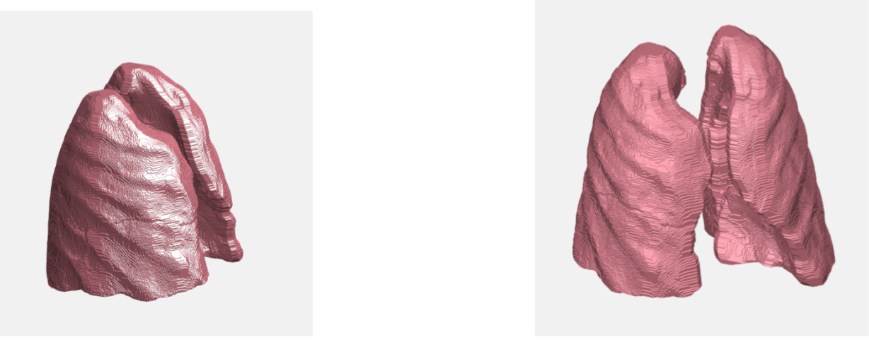 Figure 6: Final Lung Segmentation
7. Animation
The animation displays a 360 degree rotation of the segmented lung volume (Figure 7). The location of the slice moving through the image corresponds to the CT image slice used to create it. The location of the slice corresponds to the raw CT image displayed on the right of the figure. Each frame displays one slice of the CT image while the 3D volume is rotated by one degree. The animation was done with the built in MatLab VideoWriter object.
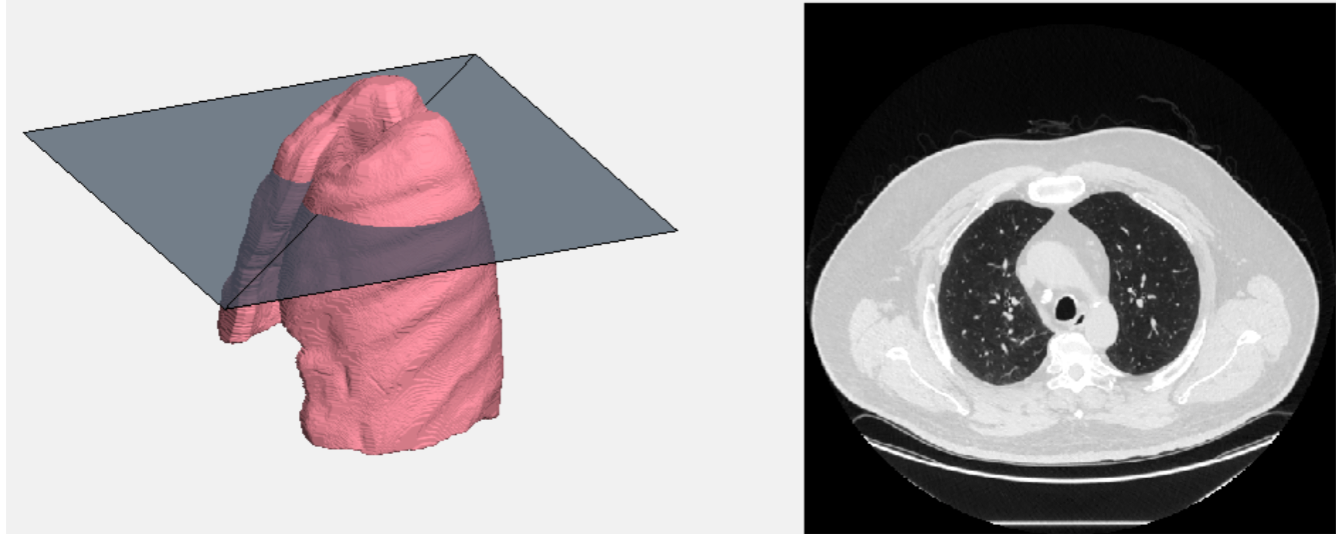 Figure 7: Still Frame from Video
Figure 3: Segmented CT Slice
Figure 4: Volume Filtered CT Slice
Figure 5: Smoothed CT with Trachea Removed
Figure 6: Final Lung Segmentation
Figure 7: Still Frame from Video